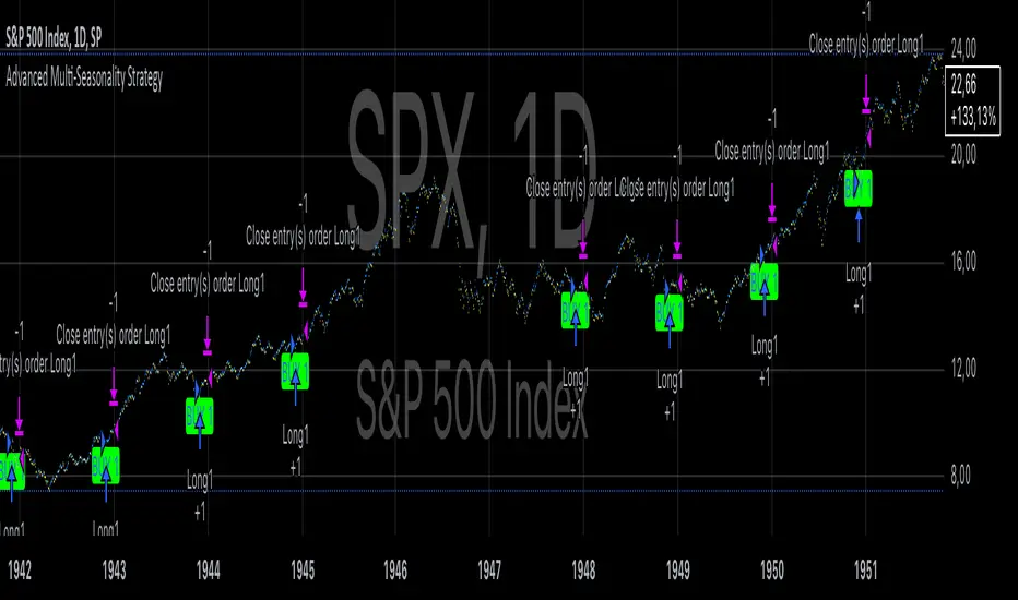
Advanced Multi-Seasonality StrategyThe Multi-Seasonality Strategy is a trading system based on seasonal market patterns. Seasonality refers to recurring market trends driven by predictable calendar-based events. These patterns emerge due to economic cycles, corporate activities (e.g., earnings reports), and investor behavior around specific times of the year. Studies have shown that such effects can influence asset prices over defined periods, leading to opportunities for traders who exploit these patterns (Hirshleifer, 2001; Bouman & Jacobsen, 2002).
How the Strategy Works:
The strategy allows the user to define four distinct periods within a calendar year. For each period, the trader selects:
Entry Date (Month and Day): The date to enter the trade.
Holding Period: The number of trading days to remain in the trade after the entry.
Trade Direction: Whether to take a long or short position during that period.
The system is designed with flexibility, enabling the user to activate or deactivate each of the four periods. The idea is to take advantage of seasonal patterns, such as buying during historically strong periods and selling during weaker ones. A well-known example is the "Sell in May and Go Away" phenomenon, which suggests that stock returns are higher from November to April and weaker from May to October (Bouman & Jacobsen, 2002).
Seasonality in Financial Markets:
Seasonal effects have been documented across different asset classes and markets:
Equities: Stock markets tend to exhibit higher returns during certain months, such as the "January effect," where prices rise after year-end tax-loss selling (Haugen & Lakonishok, 1987).
Commodities: Agricultural commodities often follow seasonal planting and harvesting cycles, which impact supply and demand patterns (Fama & French, 1987).
Forex: Currency pairs may show strength or weakness during specific quarters based on macroeconomic factors, such as fiscal year-end flows or central bank policy decisions.
Scientific Basis:
Research shows that market anomalies like seasonality are linked to behavioral biases and institutional practices. For example, investors may respond to tax incentives at the end of the year, and companies may engage in window dressing (Haugen & Lakonishok, 1987). Additionally, macroeconomic factors, such as monetary policy shifts and holiday trading volumes, can also contribute to predictable seasonal trends (Bouman & Jacobsen, 2002).
Risks of Seasonal Trading:
While the strategy seeks to exploit predictable patterns, there are inherent risks:
Market Changes: Seasonal effects observed in the past may weaken or disappear as market conditions evolve. Increased algorithmic trading, globalization, and policy changes can reduce the reliability of historical patterns (Lo, 2004).
Overfitting: One of the risks in seasonal trading is overfitting the strategy to historical data. A pattern that worked in the past may not necessarily work in the future, especially if it was based on random chance or external factors that no longer apply (Sullivan, Timmermann, & White, 1999).
Liquidity and Volatility: Trading during specific periods may expose the trader to low liquidity, especially around holidays or earnings seasons, leading to slippage and larger-than-expected price swings.
Economic and Geopolitical Shocks: External events such as pandemics, wars, or political instability can disrupt seasonal patterns, leading to unexpected market behavior.
Conclusion:
The Multi-Seasonality Strategy capitalizes on the predictable nature of certain calendar-based patterns in financial markets. By entering and exiting trades based on well-established seasonal effects, traders can potentially capture short-term profits. However, caution is necessary, as market dynamics can change, and seasonal patterns are not guaranteed to persist. Rigorous backtesting, combined with risk management practices, is essential to successfully implementing this strategy.
References:
Bouman, S., & Jacobsen, B. (2002). The Halloween Indicator, "Sell in May and Go Away": Another Puzzle. American Economic Review, 92(5), 1618-1635.
Fama, E. F., & French, K. R. (1987). Commodity Futures Prices: Some Evidence on Forecast Power, Premiums, and the Theory of Storage. Journal of Business, 60(1), 55-73.
Haugen, R. A., & Lakonishok, J. (1987). The Incredible January Effect: The Stock Market's Unsolved Mystery. Dow Jones-Irwin.
Hirshleifer, D. (2001). Investor Psychology and Asset Pricing. Journal of Finance, 56(4), 1533-1597.
Lo, A. W. (2004). The Adaptive Markets Hypothesis: Market Efficiency from an Evolutionary Perspective. Journal of Portfolio Management, 30(5), 15-29.
Sullivan, R., Timmermann, A., & White, H. (1999). Data-Snooping, Technical Trading Rule Performance, and the Bootstrap. Journal of Finance, 54(5), 1647-1691.
This strategy harnesses the power of seasonality but requires careful consideration of the risks and potential changes in market behavior over time.
Pesquisar nos scripts por "the strat"
Statistical ArbitrageThe Statistical Arbitrage Strategy, also known as pairs trading, is a quantitative trading method that capitalizes on price discrepancies between two correlated assets. The strategy assumes that over time, the prices of these two assets will revert to their historical relationship. The core idea is to take advantage of mean reversion, a principle suggesting that asset prices will revert to their long-term average after deviating significantly.
Strategy Mechanics:
1. Selection of Correlated Assets:
• The strategy focuses on two historically correlated assets (e.g., equity index futures like Dow Jones Mini and S&P 500 Mini). These assets tend to move in the same direction due to similar underlying fundamentals, such as overall market conditions. By tracking their relative prices, the strategy seeks to exploit temporary mispricings.
2. Spread Calculation:
• The spread is the difference between the prices of the two assets. This spread represents the relationship between the assets and serves as the basis for determining when to enter or exit trades.
3. Mean and Standard Deviation:
• The historical average (mean) of the spread is calculated using a Simple Moving Average (SMA) over a chosen period. The strategy also computes the standard deviation (volatility) of the spread, which measures how far the spread has deviated from the mean over time. This allows the strategy to define statistically significant price deviations.
4. Entry Signal (Mean Reversion):
• A buy signal is triggered when the spread falls below the mean by a multiple (e.g., two) of the standard deviation. This indicates that one asset is temporarily undervalued relative to the other, and the strategy expects the spread to revert to its mean, generating profits as the prices converge.
5. Exit Signal:
• The strategy exits the trade when the spread reverts to the mean. At this point, the mispricing has been corrected, and the profit from the mean reversion is realized.
Academic Support:
Statistical arbitrage has been widely studied in finance and economics. Gatev, Goetzmann, and Rouwenhorst’s (2006) landmark study on pairs trading demonstrated that this strategy could generate excess returns in equity markets. Their research found that by focusing on historically correlated stocks, traders could identify pricing anomalies and profit from their eventual correction.
Additionally, Avellaneda and Lee (2010) explored statistical arbitrage in different asset classes and found that exploiting deviations in price relationships can offer a robust, market-neutral trading strategy. In these studies, the strategy’s success hinges on the stability of the relationship between the assets and the timely execution of trades when deviations occur.
Risks of Statistical Arbitrage:
1. Correlation Breakdown:
• One of the primary risks is the breakdown of correlation between the two assets. Statistical arbitrage assumes that the historical relationship between the assets will hold in the future. However, market conditions, company fundamentals, or external shocks (e.g., macroeconomic changes) can cause these assets to deviate permanently, leading to potential losses.
• For instance, if two equity indices historically move together but experience divergent economic conditions or policy changes, their prices may no longer revert to the expected mean.
2. Execution Risk:
• This strategy relies on efficient execution and tight spreads. In volatile or illiquid markets, the actual price at which trades are executed may differ significantly from expected prices, leading to slippage and reduced profits.
3. Market Risk:
• Although statistical arbitrage is designed to be market-neutral (i.e., not dependent on the overall market direction), it is not entirely risk-free. Systematic market shocks, such as financial crises or sudden shifts in market sentiment, can affect both assets simultaneously, causing the spread to widen rather than revert to the mean.
4. Model Risk:
• The assumptions underlying the strategy, particularly regarding mean reversion, may not always hold true. The model assumes that asset prices will return to their historical averages within a certain timeframe, but the timing and magnitude of mean reversion can be uncertain. Misestimating this timeframe can lead to extended drawdowns or unrealized losses.
5. Overfitting:
• Over-reliance on historical data to fine-tune the strategy parameters (e.g., the lookback period or standard deviation thresholds) may result in overfitting. This means that the strategy works well on past data but fails to perform in live markets due to changing conditions.
Conclusion:
The Statistical Arbitrage Strategy offers a systematic and quantitative approach to trading that capitalizes on temporary price inefficiencies between correlated assets. It has been proven to generate returns in academic studies and is widely used by hedge funds and institutional traders for its market-neutral characteristics. However, traders must be aware of the inherent risks, including correlation breakdown, execution risks, and the potential for prolonged deviations from the mean. Effective risk management, diversification, and constant monitoring are essential for successfully implementing this strategy in live markets.

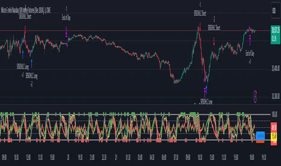
Stochastic RSI OHLC StrategyThe script titled "Stochastic RSI High Low Close Bars" is a versatile trading strategy implemented in Pine Script, designed for TradingView. Here's an overview of its features:
Description
This strategy leverages the Stochastic RSI to determine entry and exit signals in the market, focusing on high, low, and close values of the indicator. It incorporates various trading styles, stop-loss mechanisms, and multi-timeframe analysis to adapt to different market conditions.
Key Features
Stochastic RSI Analysis:
Uses the Stochastic RSI to identify potential entry points for long and short positions.
Tracks high, low, and close values for more granular analysis.
Multiple Trading Styles:
Supports diverse trading styles like Volume Color Swing, RSI Divergence, RSI Pullback, and more.
Allows switching between these styles to suit market dynamics.
Session-Based Trading:
Offers session control, limiting trades to specific hours (e.g., NY sessions).
Can close all positions at the end of the trading day.
Stop-Loss and Take-Profit Mechanisms:
Includes both static and dynamic stop-losses, with options for time-based stops, trailing stops, and momentum-based exits.
Customizable take-profit levels ensure efficient trade management.
Volume Analysis:
Integrates volume indicators to add a bias for trade entries and exits, enhancing signal reliability.
Multi-Timeframe Integration:
Employs multi-timeframe RSI analysis, allowing the strategy to capture broader trends and optimize entries.
This script is designed to provide flexibility and adaptability, making it useful for different trading strategies and market conditions. It is suitable for traders looking to refine their entries and exits with a focus on the Stochastic RSI.
Support Resistance Pivot EMA Scalp Strategy [Mauserrifle]A strategy that creates signals based on: pivots, EMA 9+20, RSI, ATR, VWAP, wicks and volume.
The strategy is developed as a helper for quick long option scalping. This strategy is primarily designed for intraday trading on the 2m SPY chart with extended hours. However, users can adapt it for use on different symbols and timeframes. These signals are meant as a helper rather than fully automated trading bots.
One of the key elements is its pivot-based calculation, driven by my integrated indicator "Support and Resistance Pivot Points/Lines ". It enables multi-timeframe pivot calculations which are used to generate the signals and offers customizability, allowing you to define rounding methods and cooldown periods to refine pivot levels. The pivots, in combination with EMA crossovers, VWAP trend, and additional filters (RSI, ATR, VWAP, wicks and volume), create an entry and exit strategy for scalping opportunities that is useful for 0/1 DTE options with an average trade time of six minutes with the default setup for SPY. Option trading should be done outside TradingView. At this moment of release there is no option trading support.
All parameters used in the strategy are tweaked based on deep backtests results and real-time behavior. Be mindful that past performance does not guarantee future results.
The strategy is designed for intermediate and advanced users who are familiar intraday option scalping techniques.
How It Works
The strategy identifies entries based on multiple conditions, including: recently above pivot, recent EMA crossovers, RSI range, candle patterns, and VWAP uptrend. It avoids trades below the VWAP lower band due to poor backtesting results in those conditions. It creates a great number of signals when it detects an uptrend, which entails: VWAP and its lower/upper band slopes are going up, and the number of next high pivot points is greater than the number of lower pivot points. This indicates that we hope it will keep going up. In historical testing, this showed favorable results. This uptrend criteria runs on 15m charts max (where up to the VWAP effectiveness is the greatest).
The strategy also checks for candle and volume patterns, identified in backtesting to improve entry levels on historic data. Which include:
A red candle after multiple green ones, hoping to jump on a trend during a small pullback
Zero lower wick
Percentage and volume is up after lower volume candles
Percentage is up and the first and second EMA slopes are going up
Percentage is up, the first EMA is higher than the second, the price low is below the second EMA and price close above it
The VWAP uptrend overrules the candle and volume conditions (thus lots of signals during those moments).
The above is the base for many signals. There is a strict mode that adds extra checks such as:
not trading when there is no next low or high pivot
requiring a VWAP uptrend only
minimum candle percentages
This mode is for analyzing history and seeing performance during these conditions. It is worth it to create a separate alert for strict mode so you are aware of these conditions during trading.
When no stop has been defined, exits will always happen on pivot crossunder confirmations. If a stop is defined (default config), the strategy exits a position when:
the position is negative or no trail has been set
at least 1 bar has past
OR no stop has been defined (overrules previous)
trail has not been activated
The second exit condition happens when the close is below first EMA(9 by default) and when:
the position has been above first EMA
the gap between close and last pivot isn't small
the position is negative or no trail has been set
OR no stop has been defined (overrules above)
trail has not been activated
There are some more variations on this but the above are the most common. These exit conditions are a safety net because the strategy heavily relies on and favors stops. The settings allow changing stops, profit takers and trails. You can configure it to always sell without the conditions above.
The script will paint the pivot lines, trailing activation/stops, EMAs and entry/exits; with extra information in the data panel. For a complete view add VWAP and RSI to your chart, which are available from TradingView official indicator library. The strategy will not rely on those added indicators since VWAP and RSI are programmed in. You can add them to track the behavior of the signals based on these filters you have configured and have a complete view trading this strategy.
As mentioned earlier, the default settings are built for SPY 2m charts, with extended hours and real-time data. Open the strategy on this chart to study how all input parameters are used. If you don't have real-time data you need to adjust the minimum volume settings (set it to 0 at first).
The backtest
The default backtest configuration is set up to simulate SPY option trading.
Start capital is set to 10,000 and we risk around 5% of that per trade (1 contract)
Commission is set to 0.005%. The reason: at the time of this publication the SPY index price is approximately $580. Two ITM 0/1 DTE options contracts, each priced around $280, which is approximately $560. The typical commission for such a trade is around $3. To simulate this commission in the backtest on the SPY index itself, a commission of 0.005% per trade has been applied, approximating the options trading costs.
Slippage of 3 is set reflecting liquid SPY
The bar magnifier feature is turned on to have more realistic fills
Trading
In backtesting, setting commission and slippage to 0 on the SPY 2m chart shows many trades result around breaking even. Personally, I view them as an opportunity and safety net to help manage emotional decisions for exits. The signals are designed for short option scalps, allowing traders to take small profits and potentially re-enter during the strategy’s position window. It's advisable to take small potential profits, such as 4%, whenever the opportunity arises and consider re-entering if the setup still looks favorable, for example price still above ema9. Exiting a long position below ema9 is a common strategy for 2m scalping.
The average trade duration is approximately 6 minutes (3 bars). The choice between ITM (in-the-money), ATM (at-the-money), or OTM (out-of-the-money) options will depend on your trading style. Personally, I’ve seen better results with ITM options because they tend to move more in sync with the underlying index, thanks to their higher delta.
It’s important to note that the signals are designed to be a helper for manual trading rather than to automate a bot. Users are encouraged to take small profits and re-enter positions if favorable conditions persist. Be mindful that past performance does not guarantee future results.
For the default SPY setup the losses will mostly be 4-10% for ITM options. Be mindful of extreme volatile conditions where losses may reach 30% quickly, especially when trading ATM/OTM options.
The following settings can be changed:
8 pivot timeframes with left/right bars and days rendered
Here you can configure the timeframes for the pivots, which are crucial. The strategy wants that a crossover has happened recently (so it might enter after a crossunder if the crossover was recent) or the price is still above the crossed pivot.
When you decide to use a pivot timeframe higher than your chart, make sure it aligns the same starting point as the chart timeframe. As stated in the 43000478429 docs, there is a dependency between the resolution and the alignment of a starting point:
1–14 minutes — aligns to the beginning of a week
15–29 minutes — aligns to the beginning of a month
from 30 minutes and higher — aligns to the beginning of a year
This alignment also affects the setting of rendered days. I recommend a max value of 5 days for 1-14 minutes timeframes.
Also make sure a higher pivot timeframe can be divided by the lower. For instance I had repaint issues using 3m pivots on a 2m chart. But 4m pivots work fine.
Please look up docs 43000478429 to make sure this information is still up to date.
Pivot rounding
The pivot rounding option is used to add pivots based on a rounded price and limit the number of pivots. While this feature is disabled by default it can be useful with tweaking strategy variations, because many orders are placed at rounded levels and tend to act as strong price barriers.
There are multiple rounding methods: round, ceil/floor, roundn (decimal) and rounding to the minimal tick.
The next feature is a powerful extension called "Cooldown rounding":
Pivot cooldown rounding
This rounds new pivot levels for a cooldown period to keep the previous pivot line instead of adding a new line when they match the rounded value within the cooldown period. The existing line will be extended. This feature is useful because it makes sure the initial line is added to the exact high/low pivot level but any future lines within the rounding will just extend the existing line. This limits the number of pivots while still having precise levels (which normal rounding lacks) and allows more precise pivot trading.
This feature also helps ensure that the number of rendered lines will not exceed 500 too much, which is the render limit on TradingView.
You can set a maximum minutes for the cooldown. The default is 3 years which will enable the cooldown rounding permanently on the intraday (due to the max bar limit).
Pivot always added when new higher/lower pivot
When using cooldown rounding, one may find it useful to override this behavior when a new lower or higher pivot level has been reached. When enabled the new level will be added despite the fact that they may be rounded the same in the cooldown check. This is a good balance between limiting pivots but also allowing preciser trading.
VWAP bands multiplier
This is used to tweak the inner VWAP working for the upper and lower band. The default VWAP multiplier (0.9) is set based on backtesting since it performed better on historic data (the strategy does not trade below the lowerband). When you add the VWAP indicator from the TradingView library to the chart, make sure it uses the same multiplier setting as within this strategy so you have a correct view of the conditions the strategy acts on.
ATR EMA smoothing length
Used to tweak the ATR EMA smoothing. By default it is set up to 4 based on deep backtesting historic data.
EMA lengths
Changing the EMA length allows you to fine tune the EMA crossing behavior. By default the strategy is set up to EMA 9 and 20 which are considered commonly used values on the 2-minute chart.
Trading intraday time restrictions
For intraday charts you can configure when the strategy starts trading after market open and when it stops, including a hard sell. This makes sure there are no open positions left for the day during backtesting and can also aid in your trading style. For example some scalpers will not trade in the first two hours. Having no signals during this time can be beneficial. It is possible to configure these settings based on the number of bars or minutes.
Not trading on days the market closes earlier
By default the strategy does not trade on days the market closes earlier in the US. This makes sure there are no open positions left open during backtesting. Make sure to change it when using it on such a day. The days are: day before independence day, day after thanksgiving, Christmas eve and new years eve.
Not trading below VWAP lowerband
Backtesting has shown poor performance when trading below the VWAP lowerband but you are free to allow it to trade in such conditions. Past performance does not guarantee future results.
Minimum volume
A minimum volume can be set up. The current value is based on better deep backtest results for SPY using real-time data (48000). When you do not have a data plan for SPY, please set it to 0 and tweak based on backtests.
Minimum ATRP
The strategy has shown during my trading that it is sensitive to higher ATRP values and more volatile market conditions. There is more chance the index moves and we can profit from this during option scalping (if it moves in your favor). The default is based on SPY backtesting (0.04%), as a balance to have a lot of trades but also capture minimal movement.
RSI range
A RSI range can be set using a minimum and maximum value so we can limit trading during overbought/oversold conditions. Backtesting for SPY has shown the strategy performs better on historic data within a tighter range, so a default range has been set to 40-65.
Allow orders on every tick (no effect on stop/profit/trail)
This setting is used to allow orders on every tick. The strategy has been developed without trading on every tick but you can change this, for example when you have configured a setup different than the default configuration that you know works well with this. The default setup will not work well with it due to too many constant signals.
Stop percentage + ATRP threshold
One of the most important settings for managing the risk. I recommend setting a stop percentage first and later the ATRP threshold where the stop is calculated based on the current ATRP value. The calculated value will only be in effect when it is greater than the normal stop--the normal stop acts as baseline. The default stop is low (0.03). With a default ATRP threshold stop of 1.12, the calculated value overrules the normal stop when the value is greater. 0.03 acts as a minimum value but in reality the stop will most likely be higher on average for SPY with the default ATRP threshold.
For the default SPY setup the losses will be around 4-10% for ITM options. Be mindful of extreme volatile conditions where losses may reach 30% quickly, especially when trading ATM/OTM options.
Profit taker percentage + ATRP threshold
Same principles as the stop percentage above, but for profit taking. There is a very high ATRP threshold of 4 set by default. Backtests showed that trailing stops perform better on historic data.
Trailing stop
Used to set up a trailing stop. A useful feature to secure profit after a run-up, or get out with a small loss after initial activation. It is important to not use too tight values because they will give unrealistic backtest results and trigger too fast in real-time. Both the trail activation level and trail stop itself can be configured with a percentage value and ATRP value. I recommend setting up the ATRP last. By default the values are 0.05 for activation and 0.03 for the stop based on SPY real-time behavior.
Always sell on pivot crossunder confirmation
The strategy includes pivot crossunder confirmations as sell condition. By default it will not sell on every crossunder confirmation but checks for different conditions (explained in detail earlier in this description). You can change this behavior.
Always sell below first EMA when position has been above
The strategy sells below the first EMA when the position has been above it. By default it will not always sell but checks for different conditions (mentioned earlier in this description). You can change this behavior.
Buy modes pivot
By default the strategy buys between pivots as long as there has been a pivot crossover and EMAs crossover recently or price is still above it. You can change the behavior so it only buys on pivot crossovers or pivot crossover confirmations. Backtesting on the default setup shows decreased performance but for other strategy variations and pivot setups this feature can be useful since many scalpers do not buy between pivots.
Strict mode
There is a strict mode that adds extra checks such as not trading when there is no next low or high pivot, requiring a VWAP uptrend only and minimum candle percentages. This mode is for analyzing history and seeing performance during these conditions. It is worth it to create a separate alert for strict mode so you are aware of these conditions during trading. The deep backtests improved with these setting but past performance does not guarantee future results.
In the strict mode section you can override the stop, minimum ATRP, set up a minimum percentage, only trade VWAP uptrends and to not trade candles without a wick.
A summary and some extra detail
At the time of release only long trades are supported
The strategy is meant for quick scalping but one might find other uses for it
Enable extended hours on intraday charts so it captures more pivots
It does not trade extended hours (pre and post market) since options do not trade during those times
real-time data is recommended and required if a symbol has delayed data by default
You can configure that it trades minutes after market open and hard sells minutes after market open
The entries have a specific label text, example: "833 LE1 / 569.71 / P:569.8". This means: / / . The condition number is only for development/debug purposes for me when you have an issue.
The strategy cannot be tweaked to work on multiple symbols and timeframes with a single config. So you will have to make a config for every timeframe and symbol. I recommend using the Indicator Templates feature of TradingView. This way you can save the settings per timeframe and symbol
The strategy is per default config very dependent on (trailing) stops because it trades between pivots too. It wants that a pivot and EMA crossover has happened more recently than a crossunder. But you can change this behavior to always force crossover buys and crossunder sells.
It’s recommended to set up alerts to notify you of entry and exit signals. Watching the chart alone might cause you to miss trades, especially in fast-moving markets.
Only a max of 500 lines can be rendered on the chart, but the strategy will function with more under the hood. When you exceed 500 you will notice the beginning of the chart has no pivots, but beneath everything functions for backtesting.
Changing settings
Changing the settings for a different symbol and/or timeframe can be a challenging task. Here's a how-to you could use the first time to help you get going:
Set commission and slippage to 0. I prefer to do this so it is more clear whether you are balancing on break-even trades
Enable the pivot timeframe equal or above your chart timeframe. Avoid repainting as discussed earlier by choosing timeframes that align with the same timeframe
Set all volume, ATR, stop, profit takers and trail values to 0
Make sure strict mode is disabled at the bottom of the settings
You now have a clean state and you should see the backtest results purely based on pivot and EMA conditions
Tweak the stop and profit taker, beginning with the simple values and then ATRP threshold
At the last moment tweak the trailing stops. Tight trailing stops create an unrealistic backtest so you will need to tweak them based on real-time behavior of the symbol you're using which you will have to monitor during signals while the market is open. The default values are low (2m intraday SPY). Only with the bar magnifier feature it is somewhat possible to tweak realistic with history data. The tighter they are, the more unrealistic your backtest results. As a starting point, set the trailing stop low and find the highest activation level that doesn't change the results drastically, then increase the stop to the value you think reflects real-time behavior.
Keep refining by testing it during real-time behavior. Does it exit too early according to your own judgment? You need to increase the stop and maybe the activation level.
I hope you will find this useful!
DISCLAIMER
Trading is risky & most day traders lose money. This indicator is purely for informational & educational purposes only. Past performance does not guarantee future results.

Chande Momentum Oscillator StrategyThe Chande Momentum Oscillator (CMO) Trading Strategy is based on the momentum oscillator developed by Tushar Chande in 1994. The CMO measures the momentum of a security by calculating the difference between the sum of recent gains and losses over a defined period. The indicator offers a means to identify overbought and oversold conditions, making it suitable for developing mean-reversion trading strategies (Chande, 1997).
Strategy Overview:
Calculation of the Chande Momentum Oscillator (CMO):
The CMO formula considers both positive and negative price changes over a defined period (commonly set to 9 days) and computes the net momentum as a percentage.
The formula is as follows:
CMO=100×(Sum of Gains−Sum of Losses)(Sum of Gains+Sum of Losses)
CMO=100×(Sum of Gains+Sum of Losses)(Sum of Gains−Sum of Losses)
This approach distinguishes the CMO from other oscillators like the RSI by using both price gains and losses in the numerator, providing a more symmetrical measurement of momentum (Chande, 1997).
Entry Condition:
The strategy opens a long position when the CMO value falls below -50, signaling an oversold condition where the price may revert to the mean. Research in mean-reversion, such as by Poterba and Summers (1988), supports this approach, highlighting that prices often revert after sharp movements due to overreaction in the markets.
Exit Conditions:
The strategy closes the long position when:
The CMO rises above 50, indicating that the price may have become overbought and may not provide further upside potential.
Alternatively, the position is closed 5 days after the buy signal is triggered, regardless of the CMO value, to ensure a timely exit even if the momentum signal does not reach the predefined level.
This exit strategy aligns with the concept of time-based exits, reducing the risk of prolonged exposure to adverse price movements (Fama, 1970).
Scientific Basis and Rationale:
Momentum and Mean-Reversion:
The strategy leverages the well-known phenomenon of mean-reversion in financial markets. According to research by Jegadeesh and Titman (1993), prices tend to revert to their mean over short periods following strong movements, creating opportunities for traders to profit from temporary deviations.
The CMO captures this mean-reversion behavior by monitoring extreme price conditions. When the CMO reaches oversold levels (below -50), it signals potential buying opportunities, whereas crossing overbought levels (above 50) indicates conditions for selling.
Market Efficiency and Overreaction:
The strategy takes advantage of behavioral inefficiencies and overreactions, which are often the drivers behind sharp price movements (Shiller, 2003). By identifying these extreme conditions with the CMO, the strategy aims to capitalize on the market’s tendency to correct itself when price deviations become too large.
Optimization and Parameter Selection:
The 9-day period used for the CMO calculation is a widely accepted timeframe that balances responsiveness and noise reduction, making it suitable for capturing short-term price fluctuations. Studies in technical analysis suggest that oscillators optimized over such periods are effective in detecting reversals (Murphy, 1999).
Performance and Backtesting:
The strategy's effectiveness is confirmed through backtesting, which shows that using the CMO as a mean-reversion tool yields profitable opportunities. The use of time-based exits alongside momentum-based signals enhances the reliability of the strategy by ensuring that trades are closed even when the momentum signal alone does not materialize.
Conclusion:
The Chande Momentum Oscillator Trading Strategy combines the principles of momentum measurement and mean-reversion to identify and capitalize on short-term price fluctuations. By using a widely tested oscillator like the CMO and integrating a systematic exit approach, the strategy effectively addresses both entry and exit conditions, providing a robust method for trading in diverse market environments.
References:
Chande, T. S. (1997). The New Technical Trader: Boost Your Profit by Plugging into the Latest Indicators. John Wiley & Sons.
Fama, E. F. (1970). Efficient Capital Markets: A Review of Theory and Empirical Work. The Journal of Finance, 25(2), 383-417.
Jegadeesh, N., & Titman, S. (1993). Returns to Buying Winners and Selling Losers: Implications for Stock Market Efficiency. The Journal of Finance, 48(1), 65-91.
Murphy, J. J. (1999). Technical Analysis of the Financial Markets: A Comprehensive Guide to Trading Methods and Applications. New York Institute of Finance.
Poterba, J. M., & Summers, L. H. (1988). Mean Reversion in Stock Prices: Evidence and Implications. Journal of Financial Economics, 22(1), 27-59.
Shiller, R. J. (2003). From Efficient Markets Theory to Behavioral Finance. Journal of Economic Perspectives, 17(1), 83-104.

Shark Zone Day Machine V17### **Strategy Overview: Shark Zone Day Machine V14**
The "Shark Zone Day Machine V14" is a daily breakout trading strategy designed for traders who wish to capitalize on intraday price movements based on key levels from the previous day. The strategy operates on a daily timeframe, allowing traders to execute precise entries and manage their trades effectively. It includes both long and short trading capabilities, with user-friendly inputs for customization.
### **Key Features:**
1. **Daily Breakout Logic**:
- **Long Position**: The strategy opens a long position when the price breaks above the previous day's high, indicating potential upward momentum.
- **Short Position**: The strategy opens a short position when the price drops below the previous day's low, signaling possible downward pressure.
2. **Stop Loss Management**:
- The strategy uses a fixed stop loss of 50 points, which is set at the previous day's low for long trades and 50 points above the entry for short trades.
3. **Spread Adjustment**:
- Includes an adjustable spread input to account for bid-ask differences, ensuring entries and exits are accurately calculated.
4. **Activation Controls**:
- Traders can easily enable or disable long and short trading strategies independently using input toggles.
5. **Custom Alert Integration**:
- The strategy includes alert messages configured to work seamlessly with Pine Connector. These alerts can be set up to automatically send trade signals to MT4, enabling a fully automated trading experience.
### **Automated Trading Setup via Pine Connector to MT4**
To implement this strategy for automated trading between TradingView and MT4 using Pine Connector, follow these steps:
1. **Apply the Script on TradingView**:
- Load the "Shark Zone Day Machine V14" script onto your TradingView chart and adjust the input parameters as needed, including activation toggles, spread, and stop loss settings.
2. **Set Up Alerts on TradingView**:
- Click on the `Alerts` button in TradingView.
- Under "Condition," select the strategy and choose "Any alert() function call."
- For each alert, use the predefined messages:
- **Long Entry Alert**: `"BUY_SIGNAL_7683370025173"`
- **Long Exit Alert**: `"BUY_EXIT_SIGNAL_7683370025173"`
- **Short Entry Alert**: `"SELL_SIGNAL_7683370025173"`
- **Short Exit Alert**: `"SELL_EXIT_SIGNAL_7683370025173"`
- Ensure the alert actions are set to "Notify on app" and "Show pop-up" for immediate feedback.
3. **Configure Pine Connector**:
- Pine Connector should be installed and set up on your MT4 platform. Ensure the Pine Connector ID matches the alert messages from the TradingView script.
- Configure your MT4 EA to recognize these signals and execute trades accordingly. For example, a `"BUY_SIGNAL_7683370025173"` alert from TradingView will instruct MT4 to place a buy order.
4. **Test the Setup**:
- It’s essential to test the automation in a demo account first. Monitor how trades are opened and closed on MT4 when alerts are triggered from TradingView.
- Adjust the parameters on TradingView if needed for optimal performance and minimal slippage.
### **Benefits of Automated Trading with This Strategy**:
- **Consistency**: Eliminates the potential for human error by executing trades precisely as per the strategy’s logic.
- **Speed**: Rapid response to breakout conditions, ensuring you capture opportunities as soon as they arise.
- **Flexibility**: The ability to adjust stop loss, spread, and trading size allows for quick adaptation to different market conditions.
### **Important Notes**:
- Ensure your TradingView account remains active and has real-time data enabled for accurate alerts.
- Verify that Pine Connector and MT4 settings are configured correctly to prevent missed trades or incorrect lot sizes.
- Be mindful of market conditions, as breakout strategies may perform differently during high-volatility periods.
By following this guide, you'll be able to leverage the "Shark Zone Day Machine V14" strategy to its full potential, automating your trades and optimizing your trading efficiency.

Williams %R StrategyThe Williams %R Strategy implemented in Pine Script™ is a trading system based on the Williams %R momentum oscillator. The Williams %R indicator, developed by Larry Williams in 1973, is designed to identify overbought and oversold conditions in a market, helping traders time their entries and exits effectively (Williams, 1979). This particular strategy aims to capitalize on short-term price reversals in the S&P 500 (SPY) by identifying extreme values in the Williams %R indicator and using them as trading signals.
Strategy Rules:
Entry Signal:
A long position is entered when the Williams %R value falls below -90, indicating an oversold condition. This threshold suggests that the market may be near a short-term bottom, and prices are likely to reverse or rebound in the short term (Murphy, 1999).
Exit Signal:
The long position is exited when:
The current close price is higher than the previous day’s high, or
The Williams %R indicator rises above -30, indicating that the market is no longer oversold and may be approaching an overbought condition (Wilder, 1978).
Technical Analysis and Rationale:
The Williams %R is a momentum oscillator that measures the level of the close relative to the high-low range over a specific period, providing insight into whether an asset is trading near its highs or lows. The indicator values range from -100 (most oversold) to 0 (most overbought). When the value falls below -90, it indicates an oversold condition where a reversal is likely (Achelis, 2000). This strategy uses this oversold threshold as a signal to initiate long positions, betting on mean reversion—an established principle in financial markets where prices tend to revert to their historical averages (Jegadeesh & Titman, 1993).
Optimization and Performance:
The strategy allows for an adjustable lookback period (between 2 and 25 days) to determine the range used in the Williams %R calculation. Empirical tests show that shorter lookback periods (e.g., 2 days) yield the most favorable outcomes, with profit factors exceeding 2. This finding aligns with studies suggesting that shorter timeframes can effectively capture short-term momentum reversals (Fama, 1970; Jegadeesh & Titman, 1993).
Scientific Context:
Mean Reversion Theory: The strategy’s core relies on mean reversion, which suggests that prices fluctuate around a mean or average value. Research shows that such strategies, particularly those using oscillators like Williams %R, can exploit these temporary deviations (Poterba & Summers, 1988).
Behavioral Finance: The overbought and oversold conditions identified by Williams %R align with psychological factors influencing trading behavior, such as herding and panic selling, which often create opportunities for price reversals (Shiller, 2003).
Conclusion:
This Williams %R-based strategy utilizes a well-established momentum oscillator to time entries and exits in the S&P 500. By targeting extreme oversold conditions and exiting when these conditions revert or exceed historical ranges, the strategy aims to capture short-term gains. Scientific evidence supports the effectiveness of short-term mean reversion strategies, particularly when using indicators sensitive to momentum shifts.
References:
Achelis, S. B. (2000). Technical Analysis from A to Z. McGraw Hill.
Fama, E. F. (1970). Efficient Capital Markets: A Review of Theory and Empirical Work. The Journal of Finance, 25(2), 383-417.
Jegadeesh, N., & Titman, S. (1993). Returns to Buying Winners and Selling Losers: Implications for Stock Market Efficiency. The Journal of Finance, 48(1), 65-91.
Murphy, J. J. (1999). Technical Analysis of the Financial Markets: A Comprehensive Guide to Trading Methods and Applications. New York Institute of Finance.
Poterba, J. M., & Summers, L. H. (1988). Mean Reversion in Stock Prices: Evidence and Implications. Journal of Financial Economics, 22(1), 27-59.
Shiller, R. J. (2003). From Efficient Markets Theory to Behavioral Finance. Journal of Economic Perspectives, 17(1), 83-104.
Williams, L. (1979). How I Made One Million Dollars… Last Year… Trading Commodities. Windsor Books.
Wilder, J. W. (1978). New Concepts in Technical Trading Systems. Trend Research.
This explanation provides a scientific and evidence-based perspective on the Williams %R trading strategy, aligning it with fundamental principles in technical analysis and behavioral finance.

Simple RSI stock Strategy [1D] The "Simple RSI Stock Strategy " is designed to long-term traders. Strategy uses a daily time frame to capitalize on signals generated by the Relative Strength Index (RSI) and the Simple Moving Average (SMA). This strategy is suitable for low-leverage trading environments and focuses on identifying potential buy opportunities when the market is oversold, while incorporating strong risk management with both dynamic and static Stop Loss mechanisms.
This strategy is recommended for use with a relatively small amount of capital and is best applied by diversifying across multiple stocks in a strong uptrend, particularly in the S&P 500 stock market. It is specifically designed for equities, and may not perform well in other markets such as commodities, forex, or cryptocurrencies, where different market dynamics and volatility patterns apply.
Indicators Used in the Strategy:
1. RSI (Relative Strength Index):
- The RSI is a momentum oscillator used to identify overbought and oversold conditions in the market.
- This strategy enters long positions when the RSI drops below the oversold level (default: 30), indicating a potential buying opportunity.
- It focuses on oversold conditions but uses a filter (SMA 200) to ensure trades are only made in the context of an overall uptrend.
2. SMA 200 (Simple Moving Average):
- The 200-period SMA serves as a trend filter, ensuring that trades are only executed when the price is above the SMA, signaling a bullish market.
- This filter helps to avoid entering trades in a downtrend, thereby reducing the risk of holding positions in a declining market.
3. ATR (Average True Range):
- The ATR is used to measure market volatility and is instrumental in setting the Stop Loss.
- By multiplying the ATR value by a custom multiplier (default: 1.5), the strategy dynamically adjusts the Stop Loss level based on market volatility, allowing for flexibility in risk management.
How the Strategy Works:
Entry Signals:
The strategy opens long positions when RSI indicates that the market is oversold (below 30), and the price is above the 200-period SMA. This ensures that the strategy buys into potential market bottoms within the context of a long-term uptrend.
Take Profit Levels:
The strategy defines three distinct Take Profit (TP) levels:
TP 1: A 5% from the entry price.
TP 2: A 10% from the entry price.
TP 3: A 15% from the entry price.
As each TP level is reached, the strategy closes portions of the position to secure profits: 33% of the position is closed at TP 1, 66% at TP 2, and 100% at TP 3.
Visualizing Target Points:
The strategy provides visual feedback by plotting plotshapes at each Take Profit level (TP 1, TP 2, TP 3). This allows traders to easily see the target profit levels on the chart, making it easier to monitor and manage positions as they approach key profit-taking areas.
Stop Loss Mechanism:
The strategy uses a dual Stop Loss system to effectively manage risk:
ATR Trailing Stop: This dynamic Stop Loss adjusts based on the ATR value and trails the price as the position moves in the trader’s favor. If a price reversal occurs and the market begins to trend downward, the trailing stop closes the position, locking in gains or minimizing losses.
Basic Stop Loss: Additionally, a fixed Stop Loss is set at 25%, limiting potential losses. This basic Stop Loss serves as a safeguard, automatically closing the position if the price drops 25% from the entry point. This higher Stop Loss is designed specifically for low-leverage trading, allowing more room for market fluctuations without prematurely closing positions.
to determine the level of stop loss and target point I used a piece of code by RafaelZioni, here is the script from which a piece of code was taken
Together, these mechanisms ensure that the strategy dynamically manages risk while offering robust protection against significant losses in case of sharp market downturns.
The position size has been estimated by me at 75% of the total capital. For optimal capital allocation, a recommended value based on the Kelly Criterion, which is calculated to be 59.13% of the total capital per trade, can also be considered.
Enjoy !

Overnight Positioning w EMA - Strategy [presentTrading]I've recently started researching Market Timing strategies, and it’s proving to be quite an interesting area of study. The idea of predicting optimal times to enter and exit the market, based on historical data and various indicators, brings a dynamic edge to trading. Additionally, it is integrated with the 3commas bot for automated trade execution.
I'm still working on it. Welcome to share your point of view.
█ Introduction and How it is Different
The "Overnight Positioning with EMA " is designed to capitalize on market inefficiencies during the overnight trading period. This strategy takes a position shortly before the market closes and exits shortly after it opens the following day. What sets this strategy apart is the integration of an optional Exponential Moving Average (EMA) filter, which ensures that trades are aligned with the underlying trend. The strategy provides flexibility by allowing users to select between different global market sessions, such as the US, Asia, and Europe.
It is integrated with the 3commas bot for automated trade execution and has a built-in mechanism to avoid holding positions over the weekend by force-closing positions on Fridays before the market closes.
BTCUSD 20 mins Performance
█ Strategy, How it Works: Detailed Explanation
The core logic of this strategy is simple: enter trades before market close and exit them after market open, taking advantage of potential price movements during the overnight period. Here’s how it works in more detail:
🔶 Market Timing
The strategy determines the local market open and close times based on the selected market (US, Asia, Europe) and adjusts entry and exit points accordingly. The entry is triggered a specific number of minutes before market close, and the exit is triggered a specific number of minutes after market open.
🔶 EMA Filter
The strategy includes an optional EMA filter to help ensure that trades are taken in the direction of the prevailing trend. The EMA is calculated over a user-defined timeframe and length. The entry is only allowed if the closing price is above the EMA (for long positions), which helps to filter out trades that might go against the trend.
The EMA formula:
```
EMA(t) = +
```
Where:
- EMA(t) is the current EMA value
- Close(t) is the current closing price
- n is the length of the EMA
- EMA(t-1) is the previous period's EMA value
🔶 Entry Logic
The strategy monitors the market time in the selected timezone. Once the current time reaches the defined entry period (e.g., 20 minutes before market close), and the EMA condition is satisfied, a long position is entered.
- Entry time calculation:
```
entryTime = marketCloseTime - entryMinutesBeforeClose * 60 * 1000
```
🔶 Exit Logic
Exits are triggered based on a specified time after the market opens. The strategy checks if the current time is within the defined exit period (e.g., 20 minutes after market open) and closes any open long positions.
- Exit time calculation:
exitTime = marketOpenTime + exitMinutesAfterOpen * 60 * 1000
🔶 Force Close on Fridays
To avoid the risk of holding positions over the weekend, the strategy force-closes any open positions 5 minutes before the market close on Fridays.
- Force close logic:
isFriday = (dayofweek(currentTime, marketTimezone) == dayofweek.friday)
█ Trade Direction
This strategy is designed exclusively for long trades. It enters a long position before market close and exits the position after market open. There is no shorting involved in this strategy, and it focuses on capturing upward momentum during the overnight session.
█ Usage
This strategy is suitable for traders who want to take advantage of price movements that occur during the overnight period without holding positions for extended periods. It automates entry and exit times, ensuring that trades are placed at the appropriate times based on the market session selected by the user. The 3commas bot integration also allows for automated execution, making it ideal for traders who wish to set it and forget it. The strategy is flexible enough to work across various global markets, depending on the trader's preference.
█ Default Settings
1. entryMinutesBeforeClose (Default = 20 minutes):
This setting determines how many minutes before the market close the strategy will enter a long position. A shorter duration could mean missing out on potential movements, while a longer duration could expose the position to greater price fluctuations before the market closes.
2. exitMinutesAfterOpen (Default = 20 minutes):
This setting controls how many minutes after the market opens the position will be exited. A shorter exit time minimizes exposure to market volatility at the open, while a longer exit time could capture more of the overnight price movement.
3. emaLength (Default = 100):
The length of the EMA affects how the strategy filters trades. A shorter EMA (e.g., 50) reacts more quickly to price changes, allowing more frequent entries, while a longer EMA (e.g., 200) smooths out price action and only allows entries when there is a stronger underlying trend.
The effect of using a longer EMA (e.g., 200) would be:
```
EMA(t) = +
```
4. emaTimeframe (Default = 240):
This is the timeframe used for calculating the EMA. A higher timeframe (e.g., 360) would base entries on longer-term trends, while a shorter timeframe (e.g., 60) would respond more quickly to price movements, potentially allowing more frequent trades.
5. useEMA (Default = true):
This toggle enables or disables the EMA filter. When enabled, trades are only taken when the price is above the EMA. Disabling the EMA allows the strategy to enter trades without any trend validation, which could increase the number of trades but also increase risk.
6. Market Selection (Default = US):
This setting determines which global market's open and close times the strategy will use. The selection of the market affects the timing of entries and exits and should be chosen based on the user's preference or geographic focus.

Martingale with MACD+KDJ opening conditionsStrategy Overview:
This strategy is based on a Martingale trading approach, incorporating MACD and KDJ indicators. It features pyramiding, trailing stops, and dynamic profit-taking mechanisms, suitable for both long and short trades. The strategy increases position size progressively using a Multiplier, a key feature of Martingale systems.
Key Concepts:
Martingale Strategy: A trading system where positions are doubled or increased after a loss to recover previous losses with a single successful trade. In this script, the position size is incremented using a Multiplier for each addition.
Pyramiding: Allows adding to existing trades when market conditions are favorable, enhancing profitability during trends.
Settings:
Basic Inputs:
Initial Order: Defines the starting size of the position.
Default: 150.0
MACD Settings: Customize the fast, slow, and signal smoothing lengths.
Default: Fast Length: 9, Slow Length: 26, Signal Smoothing: 9
KDJ Settings: Customize the length and smoothing parameters for KDJ.
Default: Length: 14, Smooth K: 3, Smooth D: 3
Max Additions: Sets the number of additional positions (pyramiding).
Default: 5 (Min: 1, Max: 10)
Position Sizing: Percent to add to positions on favorable conditions.
Default: 1.0%
Martingale Multiplier:
Add Multiplier: This value controls the scaling of additional positions according to the Martingale principle. After each loss, a new position is added, and its size is increased by the Multiplier factor. For example, with a multiplier of 2, each new addition will be twice as large as the previous one, accelerating recovery if the price moves favorably.
Default: 1.0 (no multiplication)
Can be adjusted up to 10x to aggressively increase position size after losses.
Trade Execution:
Long Trades:
Entry Condition: A long position is opened when the MACD line crosses over the signal line, and the KDJ’s %K crosses above %D.
Additions (Martingale): After the initial long position, new positions are added if the price drops by the defined percentage, and each new addition is increased using the Multiplier. This continues up to the set Max Additions.
Short Trades:
Entry Condition: A short position is opened when the MACD line crosses under the signal line, and the KDJ’s %K crosses below %D.
Additions (Martingale): After the initial short position, new positions are added if the price rises by the defined percentage, and each new addition is increased using the Multiplier.
Exit Conditions:
Take Profit: Exits are triggered when the price reaches the take-profit threshold.
Stop Loss: If the price moves unfavorably, the position will be closed at the set stop-loss level.
Trailing Stop: Adjusts dynamically as the price moves in favor of the trade to lock in profits.
On-Chart Visuals:
Long Signals: Blue triangles below the bars indicate long entries, and green triangles mark additional long positions.
Short Signals: Red triangles above the bars indicate short entries, and orange triangles mark additional short positions.
Information Table:
The strategy displays a table with key metrics:
Open Price: The entry price of the trade.
Average Price: The average price of the current position.
Additions: The number of additional positions taken.
Next Add Price: The price level for the next position.
Take Profit: The price at which profits will be taken.
Stop Loss: The stop-loss level to minimize risk.
Usage Instructions:
Adjust the parameters to your trading style using the input settings.
The Multiplier amplifies your position size after each addition, so use it cautiously, especially in volatile markets.
Monitor the signals and table on the chart for entry/exit decisions and trade management.

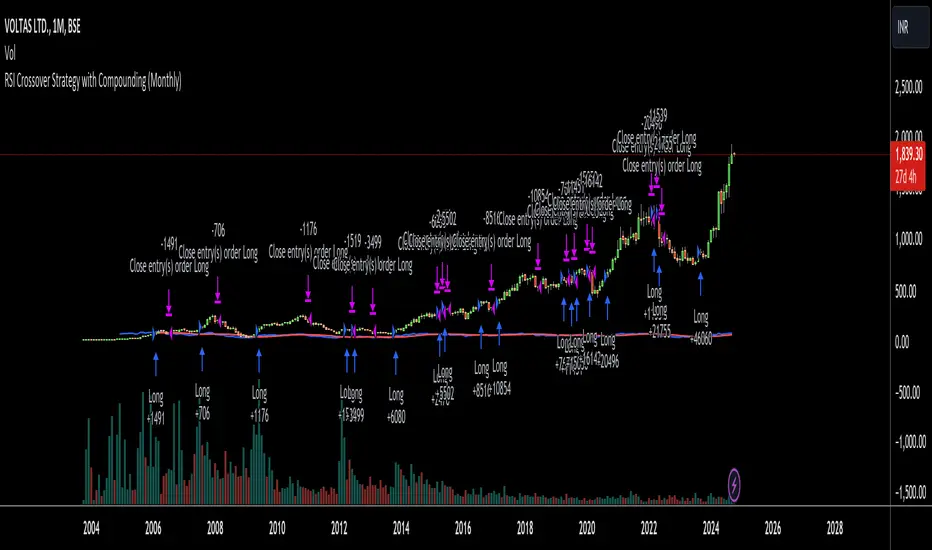
RSI Crossover Strategy with Compounding (Monthly)Explanation of the Code:
Initial Setup:
The strategy initializes with a capital of 100,000.
Variables track the capital and the amount invested in the current trade.
RSI Calculation:
The RSI and its SMA are calculated on the monthly timeframe using request.security().
Entry and Exit Conditions:
Entry: A long position is initiated when the RSI is above its SMA and there’s no existing position. The quantity is based on available capital.
Exit: The position is closed when the RSI falls below its SMA. The capital is updated based on the net profit from the trade.
Capital Management:
After closing a trade, the capital is updated with the net profit plus the initial investment.
Plotting:
The RSI and its SMA are plotted for visualization on the chart.
A label displays the current capital.
Notes:
Test the strategy on different instruments and historical data to see how it performs.
Adjust parameters as needed for your specific trading preferences.
This script is a basic framework, and you might want to enhance it with risk management, stop-loss, or take-profit features as per your trading strategy.
Feel free to modify it further based on your needs!
KAMA Cloud STIndicator:
Description:
The KAMA Cloud indicator is a sophisticated trading tool designed to provide traders with insights into market trends and their intensity. This indicator is built on the Kaufman Adaptive Moving Average (KAMA), which dynamically adjusts its sensitivity to filter out market noise and respond to significant price movements. The KAMA Cloud leverages multiple KAMAs to gauge trend direction and strength, offering a visual representation that is easy to interpret.
How It Works:
The KAMA Cloud uses twenty different KAMA calculations, each set to a distinct lookback period ranging from 5 to 100. These KAMAs are calculated using the average of the open, high, low, and close prices (OHLC4), ensuring a balanced view of price action. The relative positioning of these KAMAs helps determine the direction of the market trend and its momentum.
By measuring the cumulative relative distance between these KAMAs, the indicator effectively assesses the overall trend strength, akin to how the Average True Range (ATR) measures market volatility. This cumulative measure helps in identifying the trend’s robustness and potential sustainability.
The visualization component of the KAMA Cloud is particularly insightful. It plots a 'cloud' formed between the base KAMA (set at a 100-period lookback) and an adjusted KAMA that incorporates the cumulative relative distance scaled up. This cloud changes color based on the trend direction — green for upward trends and red for downward trends, providing a clear, visual representation of market conditions.
How the Strategy Works:
The KAMA Cloud ST strategy employs multiple KAMA calculations with varying lengths to capture the nuances of market trends. It measures the relative distances between these KAMAs to determine the trend's direction and strength, much like the original indicator. The strategy enhances decision-making by plotting a 'cloud' formed between the base KAMA (set to a 100-period lookback) and an adjusted KAMA that scales according to the cumulative relative distance of all KAMAs.
Key Components of the Strategy:
Multiple KAMA Layers: The strategy calculates KAMAs for periods ranging from 5 to 100 to analyze short to long-term market trends.
Dynamic Cloud: The cloud visually represents the trend’s strength and direction, updating in real-time as the market evolves.
Signal Generation: Trade signals are generated based on the orientation of the cloud relative to a smoothed version of the upper KAMA boundary. Long positions are initiated when the market trend is upward, and the current cloud value is above its smoothed average. Conversely, positions are closed when the trend reverses, indicated by the cloud falling below the smoothed average.
Suggested Usage:
Market: Stocks, not cryptocurrency
Timeframe: 1 Hour
Indicator:

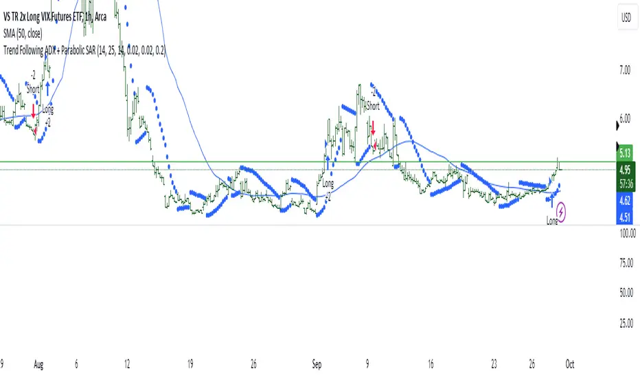
Trend Following ADX + Parabolic SAR### Strategy Description: Trend Following using **ADX** and **Parabolic SAR**
This strategy is designed to follow market trends using two popular indicators: **Average Directional Index (ADX)** and **Parabolic SAR**. The strategy attempts to enter trades when the market shows a strong trend (using ADX) and confirms the trend direction using the Parabolic SAR. Here's a breakdown:
### Key Indicators:
1. **ADX (Average Directional Index)**:
- **Purpose**: ADX measures the strength of a trend, regardless of direction.
- **Usage**: The strategy uses ADX to confirm that the market is trending. When ADX is above a certain threshold (e.g., 25), it indicates a strong trend.
- **Directional Indicators**:
- **DI+ (Directional Indicator Plus)**: Indicates upward movement strength.
- **DI- (Directional Indicator Minus)**: Indicates downward movement strength.
2. **Parabolic SAR**:
- **Purpose**: Parabolic SAR is a trend-following indicator used to identify potential reversals in the price direction.
- **Usage**: It provides specific price points above or below which the strategy confirms buy or sell signals.
### Strategy Logic:
#### **Entry Conditions**:
1. **Long Position** (Buy):
- **ADX** is above the threshold (default: 25), indicating a strong trend.
- **DI+ > DI-**, indicating the upward trend is stronger than the downward.
- The price is above the **Parabolic SAR** level, confirming the upward trend.
2. **Short Position** (Sell):
- **ADX** is above the threshold (default: 25), indicating a strong trend.
- **DI- > DI+**, indicating the downward trend is stronger than the upward.
- The price is below the **Parabolic SAR** level, confirming the downward trend.
#### **Exit Conditions**:
- Positions are closed when an opposite signal is detected.
- For example, if a long position is open and the conditions for a short position are met, the long position is closed, and a short position is opened.
### Parameters:
1. **ADX Period**: Defines the length of the period for the ADX calculation (default: 14).
2. **ADX Threshold**: The minimum value of ADX to confirm a strong trend (default: 25).
3. **Parabolic SAR Start**: The initial step for the SAR (default: 0.02).
4. **Parabolic SAR Increment**: The step increment for SAR (default: 0.02).
5. **Parabolic SAR Max**: The maximum step for SAR (default: 0.2).
### Example Trade Flow:
#### **Long Trade**:
1. ADX > 25, confirming a strong trend.
2. DI+ > DI-, indicating the market is trending upward.
3. The price is above the Parabolic SAR, confirming the upward direction.
4. **Action**: Enter a long (buy) position.
5. Exit the long position when a short signal is triggered (i.e., DI- > DI+, price below Parabolic SAR).
#### **Short Trade**:
1. ADX > 25, confirming a strong trend.
2. DI- > DI+, indicating the market is trending downward.
3. The price is below the Parabolic SAR, confirming the downward direction.
4. **Action**: Enter a short (sell) position.
5. Exit the short position when a long signal is triggered (i.e., DI+ > DI-, price above Parabolic SAR).
### Strengths of the Strategy:
- **Trend-Following**: It performs well in markets with strong trends, whether upward or downward.
- **Dual Confirmation**: The combination of ADX and Parabolic SAR reduces false signals by ensuring both trend strength and direction are considered before entering a trade.
### Weaknesses:
- **Range-Bound Markets**: This strategy may perform poorly in choppy, non-trending markets because both ADX and SAR are trend-following indicators.
- **Lagging Nature**: Since both ADX and SAR are lagging indicators, the strategy may enter trades after the trend has already started, potentially missing early profits.
### Customization:
- **ADX Threshold**: You can increase the threshold if you only want to trade in very strong trends, or lower it to capture more moderate trends.
- **SAR Parameters**: Adjusting the SAR `start`, `increment`, and `max` values will make the Parabolic SAR more or less sensitive to price changes.
### Summary:
This strategy combines the ADX and Parabolic SAR to take advantage of strong market trends. By confirming both trend strength (ADX) and trend direction (Parabolic SAR), it aims to enter high-probability trades in trending markets while minimizing false signals. However, it may struggle in sideways or non-trending markets.
For Educational purposes only !!!
Fibonacci Swing Trading BotStrategy Overview for "Fibonacci Swing Trading Bot"
Strategy Name: Fibonacci Swing Trading Bot
Version: Pine Script v5
Purpose: This strategy is designed for swing traders who want to leverage Fibonacci retracement levels and candlestick patterns to enter and exit trades on higher time frames.
Key Components:
1. Multiple Timeframe Analysis:
The strategy uses a customizable timeframe for analysis. You can choose between 4hour, daily, weekly, or monthly time frames to fit your preferred trading horizon. The high and low-price data is retrieved from the selected timeframe to identify swing points.
2. Fibonacci Retracement Levels:
The script calculates two key Fibonacci retracement levels:
0.618: A common level where price often retraces before resuming its trend.
0.786: A deeper retracement level, often used to identify stronger support/resistance areas.
These levels are dynamically plotted on the chart based on the highest high and lowest low over the last 50 bars of the selected timeframe.
3. Candlestick Based Entry Signals:
The strategy uses candlestick patterns as the only indicator for trade entries:
Bullish Candle: A green candle (close > open) that forms between the 0.618 retracement level and the swing high.
Bearish Candle: A red candle (close < open) that forms between the 0.786 retracement level and the swing low.
When these candlestick patterns align with the Fibonacci levels, the script triggers buy or sell signals.
4. Risk Management:
Stop Loss: The stop loss is set at 1% below the entry price for long trades and 1% above the entry price for short trades. This tight risk management ensures controlled losses.
Take Profit: The strategy uses a 2:1 risk-to-reward ratio. The take profit is automatically calculated based on this ratio relative to the stop loss.
5. Buy/Sell Logic:
Buy Signal: Triggered when a bullish candle forms above the 0.618 retracement level and below the swing high. The bot then places a long position.
Sell Signal: Triggered when a bearish candle forms below the 0.786 retracement level and above the swing low. The bot then places a short position.
The stop loss and take profit levels are automatically managed once the trade is placed.
Strengths of This Strategy:
Swing Trading Focus: The strategy is ideal for swing traders, targeting longer-term price moves that can take days or weeks to play out.
Simple Yet Effective Indicators: By only relying on Fibonacci retracement levels and basic candlestick patterns, the strategy avoids complexity while capitalizing on well-known support and resistance zones.
Automated Risk Management: The built-in stop loss and take profit mechanism ensures trades are protected, adhering to a strict 2:1 risk/reward ratio.
Multiple Timeframe Analysis: The script adapts to various market conditions by allowing users to switch between different timeframes (4hour, daily, weekly, monthly), giving traders flexibility.
Strategy Use Cases:
Retracement Traders: Traders who focus on entering the market at key retracement levels (0.618 and 0.786) will find this strategy especially useful.
Trend Reversal Traders: The strategy’s reliance on candlestick formations at Fibonacci levels helps traders spot potential reversals in price trends.
Risk Conscious Traders: With its 1% risk per trade and 2:1 risk/reward ratio, the strategy is ideal for traders who prioritize risk management in their trades.

Commitment of Trader %R StrategyThis Pine Script strategy utilizes the Commitment of Traders (COT) data to inform trading decisions based on the Williams %R indicator. The script operates in TradingView and includes various functionalities that allow users to customize their trading parameters.
Here’s a breakdown of its key components:
COT Data Import:
The script imports the COT library from TradingView to access historical COT data related to different trader groups (commercial hedgers, large traders, and small traders).
User Inputs:
COT data selection mode (e.g., Auto, Root, Base currency).
Whether to include futures, options, or both.
The trader group to analyze.
The lookback period for calculating the Williams %R.
Upper and lower thresholds for triggering trades.
An option to enable or disable a Simple Moving Average (SMA) filter.
Williams %R Calculation: The script calculates the Williams %R value, which is a momentum indicator that measures overbought or oversold levels based on the highest and lowest prices over a specified period.
SMA Filter: An optional SMA filter allows users to limit trades to conditions where the price is above or below the SMA, depending on the configuration.
Trade Logic: The strategy enters long positions when the Williams %R value exceeds the upper threshold and exits when the value falls below it. Conversely, it enters short positions when the Williams %R value is below the lower threshold and exits when the value rises above it.
Visual Elements: The script visually indicates the Williams %R values and thresholds on the chart, with the option to plot the SMA if enabled.
Commitment of Traders (COT) Data
The COT report is a weekly publication by the Commodity Futures Trading Commission (CFTC) that provides a breakdown of open interest positions held by different types of traders in the U.S. futures markets. It is widely used by traders and analysts to gauge market sentiment and potential price movements.
Data Collection: The COT data is collected from futures commission merchants and is published every Friday, reflecting positions as of the previous Tuesday. The report categorizes traders into three main groups:
Commercial Traders: These are typically hedgers (like producers and processors) who use futures to mitigate risk.
Non-Commercial Traders: Often referred to as speculators, these traders do not have a commercial interest in the underlying commodity but seek to profit from price changes.
Non-reportable Positions: Small traders who do not meet the reporting threshold set by the CFTC.
Interpretation:
Market Sentiment: By analyzing the positions of different trader groups, market participants can gauge sentiment. For instance, if commercial traders are heavily short, it may suggest they expect prices to decline.
Extreme Positions: Some traders look for extreme positions among non-commercial traders as potential reversal signals. For example, if speculators are overwhelmingly long, it might indicate an overbought condition.
Statistical Insights: COT data is often used in conjunction with technical analysis to inform trading decisions. Studies have shown that analyzing COT data can provide valuable insights into future price movements (Lund, 2018; Hurst et al., 2017).
Scientific References
Lund, J. (2018). Understanding the COT Report: An Analysis of Speculative Trading Strategies.
Journal of Derivatives and Hedge Funds, 24(1), 41-52. DOI:10.1057/s41260-018-00107-3
Hurst, B., O'Neill, R., & Roulston, M. (2017). The Impact of COT Reports on Futures Market Prices: An Empirical Analysis. Journal of Futures Markets, 37(8), 763-785.
DOI:10.1002/fut.21849
Commodity Futures Trading Commission (CFTC). (2024). Commitment of Traders. Retrieved from CFTC Official Website.

Advanced Position Management [Mr_Rakun]Advanced Position Management
This Pine Script code is for a strategy titled "Advanced Position Management," aimed at effective trade execution and management using multiple take profit levels, trailing stop loss, and dynamic position sizing.
Take Profit Levels: It defines up to three take profit (TP) levels, allowing partial position exits at different price thresholds. The take profit levels and their respective quantities are adjustable using inputs.
Stop Loss and Trailing Stop: The script implements an initial stop loss based on a percentage from the entry price. Additionally, it features a trailing stop that moves based on either a percentage or previous TP levels, dynamically adjusting to maximize gains while protecting profits.
Position Size: The position size is customizable and based on USD value, allowing the trader to manage risk more effectively.
Advantages:
Flexibility: Multiple take profit levels and a dynamic stop loss system allow traders to lock in profits while keeping the position open for further gains.
Risk Management: The initial stop loss and trailing stop help to limit losses and protect profits as the trade moves in the desired direction.
Automation: Once the strategy is deployed, it automatically handles entry, exit, and stop management, reducing the need for constant monitoring.
------ TR ------
Gelişmiş Pozisyon Yönetimi
Bu Pine Script kodu, Gelişmiş Pozisyon Yönetimi için kendi stratejilerinize kolayca entegre edeceğiniz bir risk yönetimidir. Çoklu kâr al seviyeleri, takip eden stop-loss ve dinamik pozisyon büyüklüğü kullanarak işlem yürütme ve yönetiminde etkilidir.
Gelişmiş Pozisyon Yönetimi
Kâr Alma Seviyeleri;
Kod, pozisyonların farklı fiyat seviyelerinde kısmi kapatılmasını sağlayan üç farklı kâr alma (TP) seviyesini tanımlar. Bu kâr alma seviyeleri ve ilgili miktarları, girişlerle ayarlanabilir.
Stop Loss ve Takip Eden Stop;
Koda, giriş fiyatından bir yüzdeye dayalı olarak başlangıçta stop-loss uygulanır. Ayrıca, fiyat hareketine göre kendini ayarlayan takip eden bir stop-loss sistemi bulunur. Ayrıca TP seviyelerini takip eden stop loss özelliğide vardır.
Avantajları:
Esneklik;
Çoklu kâr alma seviyeleri ve dinamik stop-loss sistemi, trader'ların kazançlarını kilitleyip aynı zamanda pozisyonu açık tutmalarına olanak tanır.
Risk Yönetimi;
Başlangıç stop-loss ve takip eden stop, zararı sınırlamaya ve kazançları korumaya yardımcı olur.
Otomasyon;
Strateji bir kez devreye alındığında, giriş, çıkış ve stop yönetimi otomatik olarak gerçekleştirilir, bu da sürekli takip ihtiyacını azaltır.
